Case study: state machine

This case study illustrates the use of the staircase package for analysing data derived from a state machine. States are either active or not active, and transitions between states are triggered by events. It is these events (and the time at which they occur) which comprise the data.

The data used is this case study is synthetic and fictional. Both data and the notebook for this tutorial can be obtained from the github site.

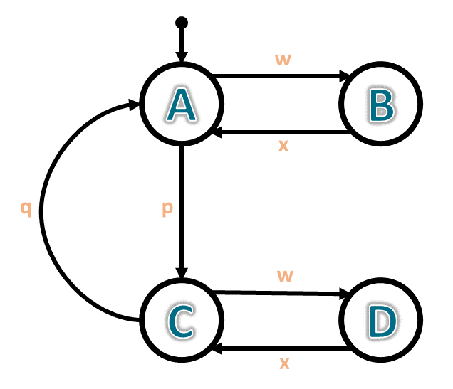
The state machine diagram is pictured below. Note that state A is the initial state (at time = 0). Note that the transitions between states A and B, and the transitions between C and D, share the same labels. This complicates the analysis, however we can still derive the results with some step function arithmetic!

import pandas as pd
import staircase as sc

We begin by importing the event data into a pandas.DataFrame instance. Each row corresponds to an event. The first column identifies the event type, while the second column gives the time (as some unspecified unit of time past 0) at which the event occurred.

data = pd.read_csv('./data/state_machine.csv')
data

/home/docs/checkouts/readthedocs.org/user_builds/railing/envs/v1.6.4/lib/python3.8/site-packages/ipykernel/ipkernel.py:283: DeprecationWarning: `should_run_async` will not call `transform_cell` automatically in the future. Please pass the result to `transformed_cell` argument and any exception that happen during thetransform in `preprocessing_exc_tuple` in IPython 7.17 and above.
  and should_run_async(code)

	event	time
0	w	14.5
1	x	14.7
2	w	32.8
3	x	40.9
4	p	55.0
...	...	...
994	w	9545.0
995	x	9551.5
996	p	9559.8
997	w	9566.2
998	x	9567.2

999 rows × 2 columns

If the transition from A to B, and B to A, were instead labelled y and z respectively, then analysing with staircase would be straightforward. For example, a binary-valued step function representing when state B is active could be obtained with the following code:

We will take a similar approach but we will need to appeal to compound states - a state composed of multiple substates. We will denote the compound state AB as meaning in state A or B, and likewise for compound states CD and BD.

Compound state AB becomes active whenever event q occurs, and becomes inactive when event p occurs. Also note that we start in AB at time = 0. We can create a step function for AB with the following code:

AB = sc.Stairs().layer(0).layer(data[data.event == "q"].time, data[data.event == "p"].time)
AB.plot()

/home/docs/checkouts/readthedocs.org/user_builds/railing/envs/v1.6.4/lib/python3.8/site-packages/ipykernel/ipkernel.py:283: DeprecationWarning: `should_run_async` will not call `transform_cell` automatically in the future. Please pass the result to `transformed_cell` argument and any exception that happen during thetransform in `preprocessing_exc_tuple` in IPython 7.17 and above.
  and should_run_async(code)

<AxesSubplot:>

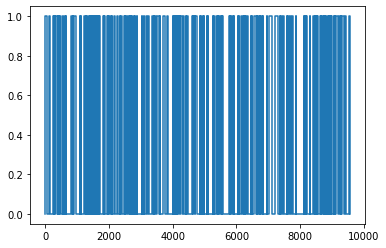
Note the first call to the layer method, increases the value of the step function from 0 to 1, at time 0. It is also important to know that there is no pairing between q and p events. In fact we start in state A, and finish in state C, and so there aren’t even an equal number of p and q events in our data (see value_counts result below). This is fine however, with the layer method simply interpreting the start parameter as times at which the step function increases by 1, and the end parameter as times at which the step function decreases by 1.

data.event.value_counts()

x    322
w    322
p    178
q    177
Name: event, dtype: int64

We can also derive step functions for compound states CD and BD like so:

CD = sc.Stairs().layer(data[data.event == "p"].time, data[data.event == "q"].time)
BD = sc.Stairs().layer(data[data.event == "w"].time, data[data.event == "x"].time)

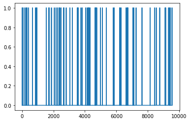
Note that unlike the singular states, it is possible to be in more than one compound state at any time. In fact it this result that our approach relies upon. If compound state AB is active, and compound state BD is active, then state B must be active (and the converse is true also). Therefore we can create a step function for state B by multiplying the step functions for AB and BD together.

B = AB*BD
B.plot()

<AxesSubplot:>

We can then obtain a step function for state A by using the fact that if state A is active, then compound state AB is active and state B is not (and the converse is true. This is equivalent to subtracting the step function for state B from the step function for compound state AB:

A = AB - B
A.plot()

<AxesSubplot:>

The same approach can be taken to derive step functions for states D and C:

D = CD*BD
C = CD - D

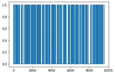
If we add the step functions for these singular states together then we obtain a step function for the compound state composed of all singular states. This step function should be zero valued and negative infinity and transitioning to a value of 1 at time = 0. We can verify this by plotting the result, remembering that the infinite length segments of a step function are not plotted:

(A + B + C + D).plot()

<AxesSubplot:>

Now that we have step functions for the singular states we can answer questions such as “what fraction of time during the first 200 time units was spent in time A?”: (38.1%)

A.mean(0,200)

0.38099999999999995